User Guide
Tutorials
The best way to get started with OpTiMSoC after you’ve prepared your system as described in the previous chapter is to follow some of our tutorials. They are written with two goals in mind: to introduce some of the basic concepts and nomenclature of manycore SoC, and to show you how those are implemented and can be used in OpTiMSoC.
Some of the tutorials (especially the first ones) build on top of each other, so it’s recommended to do them in order. Simply stop if you think you know enough to implement your own ideas!
Starting Small: Compute Tile and Embedded Software (Simulated)
It is a good starting point to simulate a single compute tile of a distributed memory system. Therefore a simple example is included and demonstrates the general simulation approach and gives an insight in the software building process.
Simulating only a single compute tile is essentially an OpenRISC core plus memory and the network adapter, where all I/O of the network adapter is not functional in this test case. It can therefore only be used to simulate local software.
You can find this example in $OPTIMSOC/examples/sim/compute_tile.
In addition to the simulated SoC hardware, you also need software that runs on the system. Our demonstration software is available in an extra repository:
git clone https://github.com/optimsoc/baremetal-apps
cd baremetal-apps
Build a simple “Hello World” example:
cd hello
make
You will then find the executable elf file as hello/hello.elf.
Furthermore some other files are built.
They are essentially transformed versions of the ELF file, i.e. the software binary.
hello.disis the disassembly of the filehello.binis the elf representation of the binary filehello.vmemis a textual copy of the binary file
Now you have everything you need to run the hello world example on a simulated SoC hardware:
$OPTIMSOC/examples/sim/compute_tile/compute_tile_sim_singlecore --meminit=hello.vmem
And you’ll get roughly this output:
[                  22, 0] Software reset
[               63128, 0] Terminated at address 0x0000e958 (status:          0)
- ../src/optimsoc_trace_monitor_trace_monitor/verilog/trace_monitor.sv:89: Verilog $finish
Furthermore, you will find a file called stdout.000 which shows the actual output:
# OpTiMSoC trace_monitor stdout file
# [TIME, CORE] MESSAGE
[               39614, 0] Hello World! Core 0 of 1 in tile 0, my absolute core id is: 0
[               48764, 0] There are 1 compute tiles:
[               57162, 0]  rank 0 is tile 0
Congratulations, you’ve ran your first OpTiMSoC system!
Note
If you are already familiar with embedded systems or microcontrollers, you might wonder: how did the printf() output from the software get into the stdout.000 file if there is no UART or anything similar?
OpTiMSoC software makes excessive use of a useful part of the OpenRISC ISA.
The “no operation” instruction l.nop has a parameter K in assembly.
This can be used for simulation purposes. It can be used for instrumentation, tracing or special purposes as writing characters with minimal intrusion or simulation termination.
The termination is forced with l.nop 0x1.
The instruction is observed and a trace monitor terminates when it was observed at all cores (shortly after main() returned).
With this method you can simply provide constants to your simulation environments.
For variables this method is extended by putting data in further registers (often r3).
This still is minimally intrusive and allows you to trace values.
The printf is also done that way (see newlib):
static void sim_putc(unsigned char c) {
    asm("l.addi r3,%0,0" : : "r" (c) : "r3");
    asm("l.nop 4");
}
This function is called from printf as write function. The trace monitor captures theses characters and puts them to the stdout file.
You can easily add your own traces using a macro defined in $OPTIMSOC/soc/sw/include/baremetal/optimsoc-baremetal.h:
#define OPTIMSOC_TRACE(id,v)                \
   asm("l.addi r3,%0,0" : : "r" (v) : "r3"); \
   asm("l.nop %0": :"K" (id));
See the Waves
One major benefit of simulating a SoC is the possibility to inspect every signal inside the hardware design quite easily.
When running a Verilator simulation, as we did in the previous step, you can simply add the --vcd command line option.
It instructs Verilator to write all signals into a file.
You can then start a waveform viewer, like GTKWave to display it.
$OPTIMSOC/examples/sim/compute_tile/compute_tile_sim_singlecore --meminit=hello.vmem --vcd
This command will run the hello world example like it did before, but this time Verilator additionally writes a sim.vcd waveform file.
You can now view this file.
gtkwave -o sim.vcd
The screenshot is similar to what you should see when running GTKWave.
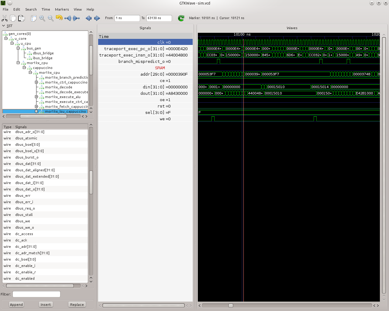
On the left side you find a hierarchy of all signals in the system. Add them to the wave view and explore all internals of a working SoC at your fingertips! Can you find the program counter? The instruction and data caches? The branch predictor?
Going Multicore: Simulate a Multicore Compute Tile
Next you might want to build an actual multicore system. In a first step, you can just start simulations of compute tiles with multiple cores.
Inside $OPTIMSOC/examples/sim/compute_tile you’ll find a dual-core version and a quad-core version of the system with just one compute tile that you just simulated in the previous step.
You can run those examples like you did before.
The first thing you observe: the simulation runs become longer.
After each run, inspect the stdout.* files.
Welcome to the multicore world!
Tiled Multicore SoC: Simulate a Small 2x2 Distributed Memory System
Next we want to run an actual NoC-based tiled multicore system-on-chip, with the examples you get system_2x2_cccc.
The nomenclature in all pre-packed systems first denotes the dimensions and then the instantiated tiles, here cccc as four compute tiles.
In our pre-built example, each compute tile has two CPU cores, meaning you have eight CPU cores in total.
Execute it again to get the hello world experience:
$OPTIMSOC/examples/sim/system_2x2_cccc/system_2x2_cccc_sim_dualcore --meminit=hello.vmem
In our simulation all cores in the four tiles run the same software. Before you shout “that’s boring”: you can still write different code depending on which tile and core the software is executed. A couple of functions are useful for that:
optimsoc_get_numct(): The number of compute tiles in the systemoptimsoc_get_numtiles(): The number of tiles (of any type) in the systemoptimsoc_get_ctrank(): Get the rank of this compute tile in this system. Essentially this is just a number that uniquely identifies a compute tile.
There are more useful utility functions like those available, find them in the file $OPTIMSOC/soc/sw/include/baremetal/optimsoc-baremetal.h.
A simple application that uses those functions to do message passing between the different tiles is hello_mpsimple.
This program uses the simple message passing facilities of the network adapter to send messages.
All cores send a message to core 0.
If all messages have been received, core 0 prints a message “Received all messages. Hello World!”.
# start from the the baremetal-apps source code directory
cd hello_mpsimple
make
$OPTIMSOC/examples/sim/system_2x2_cccc/system_2x2_cccc_sim_dualcore --meminit=hello_mpsimple.vmem
Have a look what the software does (you find the code in hello_mpsimple.c).
Let’s first check the output of core 0.
$> cat stdout.000
# OpTiMSoC trace_monitor stdout file
# [TIME, CORE] MESSAGE
[               42844, 0] Wait for 3 messages
[               48734, 0] Received all messages. Hello World!
Finally, let’s have a quick glance at a more realistic application: heat_mpsimple.
You can find it in the same place as the previous applications, hello and hello_mpsimple.
The application calculates the heat distribution in a distributed manner.
The cores coordinate their boundary regions by sending messages around.
Can you compile this application and run it?
Don’t get nervous, the simulation can take a couple of minutes to finish.
Have a look at the source code and try to understand what’s going on.
Also have a look at the stdout log files.
Core 0 will also print the complete heat distribution at the end.
Observing Software During Execution: The Debug System
Up to now, you have seen the output of the software that runs on your SoC. And you had a look deep into the inner works of the SoC by looking at the waveforms.
In a real-world system, you need something in between: a way to observe the software as it executes on a chip, but without observing or understanding all the signals inside the hardware. This is what the debug system provides: hardware inside the chip which allows you to observe what’s going on during software execution.
OpTiMSoC also comes with an extensive debug system. In this section, we’ll have a look at this system, how it works and how you can use it to debug your applications. But before diving into the details, we’ll have a short discussion of the basics which are necessary to understand the system.
Many developers know debugging from their daily work. Most of the time it involves running a program inside a debugger like GDB or Microsoft Visual Studio, setting a breakpoint at the right line of code, and stepping through the program from there on, running one instruction (or one line of code) at a time. This technique is what we call run-control debugging. While it works great for single-threaded programs, it cannot easily be applied to debugging parallel software running on possibly heterogeneous many-core SoC. Instead, the debug support in OpTiMSoC mainly relies on tracing. Tracing does not stop or otherwise influence the SoC itself; it only “records” what’s going on during software execution, and transmits this data to the developer.
The debug system consists of two main parts: the hardware part runs on the OpTiMSoC system itself and collects all data. The other part runs on a developer’s PC (often also called host PC) and controls the debugging process and displays the collected data.
After this introduction, let’s make use of the debug system to obtain various traces. Just like in the previous examples, our SoC hardware is still running in Verilator. This tutorial works best if you have multiple terminal windows open at the same time, as we’ll need to have multiple programs running at the same time.
So, open a new terminal (or a new tab inside your terminal), and start the simulation of the SoC hardware.
$OPTIMSOC/examples/sim/system_2x2_cccc/system_2x2_cccc_sim_dualcore_debug
The first and most common task using the debug system is to run a program (just like we did before with the --meminit parameter).
Open a second terminal (leave the first one running!) and type
osd-target-run -e hello.elf -vvv
The osd-target-run command takes a couple seconds to finish, so don’t get nervious.
If everything goes to plan osd-target-run just does its job: run the provided ELF file hello.elf on all CPUs in the system.
To do that, it internally performs the following steps:
Connect to the simulation over TCP (on port 23000 and 23001)
Halt all CPUs
Load all memories in the system (since this is a 2x2 system, there are four memories) with the ELF file
Reset and start all CPUs
Close the TCP connection
If you switch back to the first console where you started the simulation you should see something like this:
$> $OPTIMSOC/examples/sim/system_2x2_cccc/system_2x2_cccc_sim_dualcore_debug
Glip TCP DPI listening on port 23000 and 23001
[                  24, 0] Software reset
[                  24, 1] Software reset
[                  24, 2] Software reset
[                  24, 3] Software reset
Client connected
Disconnected
[             1035016, 0] Terminated at address 0x0000ee38 (status:          0)
[             1035016, 1] Terminated at address 0x0000ee38 (status:          0)
[             1035016, 2] Terminated at address 0x0000ee38 (status:          0)
[             1035016, 3] Terminated at address 0x0000ee38 (status:          0)
- ../src/optimsoc_trace_monitor_trace_monitor_0/verilog/trace_monitor.sv:94: Verilog $finish
- ../src/optimsoc_trace_monitor_trace_monitor_0/verilog/trace_monitor.sv:94: Verilog $finish
- ../src/optimsoc_trace_monitor_trace_monitor_0/verilog/trace_monitor.sv:94: Second verilog $finish, exiting
Just like in the previous examples you can see the output of the program runs as captured by the simulation software in the files stdout.NNN in the directory where you started the simulation.
Reading the stdout files works great as long as OpTiMSoC runs in simulation – but how can you access the program’s output when it runs on an FPGA?
The answer is called “system trace”, and you’ll learn more about that in the next section.
System Traces
System traces (sometimes also called instrumentation traces) give software developers a tool to instruct their software running on OpTiMSoC to send information into a “system trace log”.
By default, all calls to printf() result in an entry in the system trace.
(See the discussion above for how this works.)
This system trace log can then be captured on the host and displayed.
To capture a system trace from the system we’ll again use the osd-target-run tool:
osd-target-run -e hello.elf --systrace -vvv
Just like before, osd-target-run initializes the memories and starts the CPUs.
It then starts recording system traces until you press CTRL-C to end the trace collection.
(Yes, you need to abort the program by pressing CTRL-C! It will not terminate itself.)
After roughly 20 seconds, you can press CTRL-C to stop collecting traces.
Now you can analyze the collected traces in the same directory you ran osd-target-run in.
The files systrace.print.NNNN.log contain the printf() output of the program.
These files are generated by analyzing the raw system log events, which are recorded in systrace.NNNN.log.
Core Function Traces
If you need more insight into a program than system traces provide, or want to get insight into a program which isn’t instrumented to generate system traces, core function traces come to help. These traces are recording every call of a function and every return from it, resulting in traces which allow you to understand which parts of your program have been called.
To obtain a core trace use the following command:
osd-target-run -e hello.elf --coretrace -vvv
Just like in the previous example, you need to stop the trace collection by pressing CTRL-C.
You can then view the traces in the coretrace.NNNN.log files.
This completes our short trip through the debug system. Knowing about it will be of great help when we move on to the next step: running OpTiMSoC on an FPGA.
Our SoC on an FPGA
Welcome to the fun of real hardware! Before we can get started, you need to clarify some prerequisites.
Prerequisites: FPGA board and Vivado
This, of course, first means that you need borrow, buy or otherwise obtain an FPGA board. In this tutorial, we use the Nexys 4 DDR board by Xilinx/Digilent. It’s not that expensive (of course, depending on your financial situation) and widely available. If you need help obtaining one, let us know - maybe we can help out in some way.
Additionally you need to download and install the Xilinx Vivado tool (the cost-free WebPack license is sufficient). We used the 2016.4 version when preparing this tutorial; we strongly recommend you also use this exact version.
Once you have obtained the FPGA board, connect it to the PC on the “PROG UART” USB connection. You don’t need to connect any additional power supply.
Programming the FPGA
With the board connected, we can program (or “flash”) the FPGA with our hardware design, the bitstream. The OpTiMSoC release contains pre-built bitstreams for the single compute tile system, meaning we can start directly with programming the FPGA.
There are two ways to program the device: using the Vivado GUI, or using the command line.
Programming the FPGA with the Vivado GUI
Open Vivado (e.g. by typing
vivadointo a terminal window)On the welcome screen, click on “Hardware Manager”
Ensure that your Nexys 4 DDR board is plugged into your PC and is turned on.
Click on “Open Target” in the green bar on the top, and then on “Auto Connect”
Now click on “Program Device” in the same green bar and select the only option
xc7a100t_0(that’s the FPGA on the board).- In the dialog window, select the bitstream file. We’ll start directly with the larger 2x2 system, you can find the bitstream in
$OPTISMOC/examples/fpga/nexys4ddr/compute_tile/compute_tile_nexys4ddr_singlecore.bit.
You can leave the other field “Debug probes file” empty.
Click on “Program” to download the bitstream onto the FPGA.
After a couple of seconds, your FPGA contains the SoC hardware and is ready to be used.
Programming the FPGA on the Command Line
optimsoc-pgm-fpga $OPTIMSOC/examples/fpga/nexys4ddr/compute_tile/compute_tile_nexys4ddr_singlecore.bit xc7a100t_0
Connecting
In the previous tutorials, we have already seen the debug infrastructure and connected to it over TCP. We now use the same tools to connect to our SoC, but this time we connect to the FPGA using UART. Fortunately, you don’t need to connect any additional cables; the USB cable that you just used to program the FPGA is also the serial connection.
First, check which serial port was assigned to the board. Usually the easiest way is to do a
ls /dev/ttyUSB*
If you have only the Nexys 4 DDR board connected, you’ll see only one device, e.g. /dev/ttyUSB1.
Make note of this device name, and replace it accordingly in all the following steps in this tutorial.
Running Software
Now that you’ve connected to the system, can you run software on it?
Just like in the previous chapter we’ll use the osd-target-run tool, this time passing it some paramters to connect to the FPGA instead to a simulation.
osd-target-run -e hello.elf -b uart -o device=/dev/ttyUSB1,speed=12000000 --coretrace --systrace --verify -vvv
# let it run for a couple of seconds, then press CTRL-C to stop collecting traces
When you run software, you’ll notice two things: first, the output is the same as you’ve already seen when running the system in simulation. But: it’s much faster. The FPGA runs at 50 MHz, which is still quite slow compared to current desktop processors, but still much faster than the simulation.
Before we end, let’s discuss one more topic which helps you in writing good software for OpTiMSoC: message passing.
Make Message Passing More Simple
So far the example programs you have seen used the low level message passing buffers to exchange data between the tiles. You may remember that exchanging this data involved forming and parsing messages including the low level network-on-chip details.
To abstract from these low level details and to encapsulate certain extensions OpTiMSoC comes with the message passing library (libmp).
It is a rather simple, straight-forward message passing API.
Two different styles of communication are supported: message-oriented and connection-oriented.
Message-oriented communication is preferred when you have spurious communication between many different communication partners.
Connection-oriented communication is preferred when you have a fixed setup of channels between communication partners.
In this part of the tutorial you will learn the basic usage of the message passing library using message-oriented communication.
In the baremetal-apps you can find the hello_mp example.
Inspecting hello_mp.c you can see that it is much less code than the low level example from before.
Lets have a look at how it works. It starts with initializing the hardware and software:
optimsoc_init(0);
optimsoc_mp_initialize(0);
The parameters of those functions can be ignored for now. After calling those functions you can use the message passing library.
Communication in the message passing library takes place between so called endpoints. In the next step we create an endpoint in each tile:
optimsoc_mp_endpoint_handle ep;
optimsoc_mp_endpoint_create(&ep, 0, 0, OPTIMSOC_MP_EP_CONNECTIONLESS, 2, 0);
optimsoc_mp_endpoint_handle is the opaque type used to identify an endpoint in your code.
You create and initialize the endpoint by calling optimsoc_mp_endpoint_create() that takes a reference to this handle as first parameter.
The second and third parameter initialize the endpoint with a node and port.
Each endpoint is globally addressable with its (tile, node, port) identifier.
In our case the node 0 and port 0 endpoint is created in each tile.
The remaining parameters of optimsoc_mp_endpoint_create() configure the endpoint.
By using OPTIMSOC_MP_EP_CONNECTIONLESS we create it to receive messages from arbitrary tiles.
The last two parameters configure the number of messages it can hold and the maximum message size (0 says it is the default).
Now the code of the example diverts again, all but tile 0 execute:
optimsoc_mp_endpoint_handle ep_remote;
optimsoc_mp_endpoint_get(&ep_remote, 0, 0, 0);

optimsoc_mp_msg_send(ep, ep_remote, (uint8_t*) &rank, sizeof(rank));
So what they do is to define a second endpoint. But in this case it is not locally generated but points to a remote endpoint. It is the one we want to send a message too: tile 0, node 0, port 0. What happens under the hood it blocks until the remote endpoint is created and ready and than stores some information locally. In the final step the software sends a word to the remote endpoint using the local endpoint for sending.
In tile zero the software waits to receive all messages using:
optimsoc_mp_msg_recv(ep, (uint8_t*) &remote, 4, &received);
You can now run the example using:
# start from the the baremetal-apps source code directory
cd hello_mp
make
$OPTIMSOC/examples/sim/system_2x2_cccc/system_2x2_cccc_sim_dualcore --meminit=hello_mp.vmem
... (we've skipped some output here) ...
[               37812, 0] Event 0x0380: 0x00018c08
[               37844, 2] Event 0x0380: 0x00018c08
[               37872, 4] Event 0x0380: 0x00018c08
[               37900, 6] Event 0x0380: 0x00018c08
[               39984, 2] External interrupt exception
[               40012, 4] External interrupt exception
[               40040, 6] External interrupt exception
[               42048, 2] Return from exception
[               42076, 4] Return from exception
[               42104, 6] Return from exception
... (we've skipped some output here) ...
[              171970, 6] Event 0x0303: 0x00018d10
[              171982, 6] Event 0x0303: 0x00000000
[              172212, 6] Event 0x0304: 0x00018d10
[              172224, 6] Event 0x0304: 0x00000000
[              172240, 6] Event 0x0304: 0x00000004
[              172782, 0] External interrupt exception
[              173528, 6] Event 0x0305: 0x00018d10
[              174822, 0] Return from exception
[              174944, 6] Terminated at address 0x00011364 (status:          0)
[              185912, 0] Terminated at address 0x00011364 (status:          0)
- ../src/optimsoc_trace_monitor_trace_monitor_0/verilog/trace_monitor.sv:94: Verilog $finish
The simulation is currently very verbose, the events are emitted by the library to debug the message passing protocol.
More important is the output of tile 0 in stdout.000:
# OpTiMSoC trace_monitor stdout file
# [TIME, CORE] MESSAGE
[               72050, 0] Received from 1
[               78792, 0] Received from 2
[              179834, 0] Received from 3
Run Linux on OpTiMSoC
Up to now all software running on OpTiMSoC was “baremetal” software, similar to software run on a microcontroller. For many purposes “baremetal” software is sufficient. However, if you want to write more advanced software an operating system (OS) can help: it provides task management (scheduling), separates resources between tasks, and provides standardized interfaces which are expected by many of today’s applications (e.g. pthreads). For many, the operating system of choice is Linux, and it’s natively supported by OpTiMSoC. This tutorial section explores how to build a Linux “image,”. i.e. a binary which contains both the Linux kernel (the actual operating system), together with a root filesystem containing all userspace components.
# get the OpTiMSoC buildroot configuration (a "br2-external tree")
git clone https://github.com/optimsoc/optimsoc-buildroot.git
cd optimsoc-buildroot
OPTIMSOC_BUILDROOT_DIR=$PWD
OPTIMSOC_BUILDROOT_VERSION=$(cat $OPTIMSOC_BUILDROOT_DIR/buildroot_version)
cd .. # back to your source directory

# get buildroot itself
git clone https://git.busybox.net/buildroot
cd buildroot
git checkout $OPTIMSOC_BUILDROOT_VERSION
make BR2_EXTERNAL=$OPTIMSOC_BUILDROOT_DIR optimsoc_computetile_singlecore_defconfig
make
This leaves a file output/images/vmlinux in the buildroot directory, which is in fact a regular ELF file for OpenRISC, which can be loaded on the system like a baremetal application.
To see the output of the Linux during boot, and to have a console to interact with the Linux system we make use of the UART device emulation provided by Open SoC Debug, and built into the compute_tile designs.
To continue with this tutorial we use the compute_tile design with a with a single core and the debug system for the Nexys 4 DDR board.
You can find this design in the folder $OPTIMSOC/examples/fpga/nexys4ddr/compute_tile/compute_tile_nexys4ddr_singlecore.
# Program the FPGA on the Nexys 4 DDR board
optimsoc-pgm-fpga $OPTIMSOC/examples/fpga/nexys4ddr/compute_tile/compute_tile_nexys4ddr_singlecore.bit xc7a100t_0
Now you can load the Linux image on the FPGA.
See notes earlier in this tutorial for a discussion on the correct parameters for osd-target-run.
osd-target-run -e YOUR_BUILDROOT_DIR/output/images/vmlinux -b uart -o device=/dev/ttyUSB1,speed=12000000 --systrace -vvv
Watch the output of this command.
If all goes well the output should contain a line similar to libosd: DEM-UART pseudo-terminal available at /dev/pts/19.
Keep note of the device file (starting with /dev/pts/), you’ll need this path to connect to the Linux console on the OpTiMSoC system.
To connect, open a second terminal window on your machine, and use screen to connect to the remote console (use the appropriate device name as displayed by osd-target-run instead of /dev/pts/19):
screen /dev/pts/19
You should now see the output of Linux booting, and as soon as the boot process is done you can log into the system as root user (no password is required).
You can now interact with the system as it would be a normal Linux system.
If you have some time to spare, how about playing a round of pacman?
# convince Linux that our console supports colors
stty cols 80 rows 80
export TERM=linux

# and run pacman
/usr/games/pacman4linux
This concludes our tutorial session, and hands over to you: modify the software as you wish, program it again, analyze the simulations and explore your first multicore SoC.